Paper Walkthrough — Matrix Calculus for Deep Learning (Part 1 / 2)

Time and time again I find myself learning and forgetting matrix calculus, essentially getting nowhere. So I thought to myself, this time I’d try teaching it through a blog post and see if that helps cement my knowledge. Additionally like Rachel Thomas says, any email that’s written twice should be a blog post. While I am yet to see Matrix Calculus discussed on emails, it has taken up enough time and mental parking space to warrant a post of its own.

This walkthrough will take you through the paper, “The Matrix Calculus You Need For Deep Learning” by Terence Parr and Jeremy Howard. The intended audience is someone who wishes to get their feet wet with DL (Deep Learning) math, primarily, people like me, who learn and forget.

I assume that readers will be familiar with:

1. The foundations of Neural Networks, such as what are neurons, what are weights and biases, ReLU etc.(reference).
2. Basic differentiation and the concept of partial derivatives.

Affine Transformation

Think about the equation for a straight line, with the independent variable y and the dependent variable x:

Eq.1 : Straight Line

The output of a single neuron in a neural network is given by something similar to the above Eq.1:

Eq.2 : Output of a single neuron in a neural network

So far, so good. An affine transformation is simply a linear equation of weights and biases. The output z(x) is fed to an activation function, the ReLU (Rectified Linear Unit). This activation(x) is optimized to choose values for the weights and biases, (w and b) such that we get the lowest error possible.

Eq.3 : Comparison of the predicted and target values

We need to generalize the above equation such that we can optimize the weights and biases of all the neurons in the network to give the lowest possible error. However, we cannot do this one by one for each neuron.

Instead, we could have a matrix of weights and a matrix of the biases, which we then differentiate and equate to 0, to find out the values of the weights and biases for which the loss is the lowest.

However, we cannot use normal differentiation when we differentiate a matrix. This is where the gradient comes in.

Gradients

The gradient of a function is simply the matrix of its partial derivatives.

Eq.4 : Gradient

Consider a function f(x, y) = 10x²y². The gradient of this function would be:

Eq.5 : Gradient of the function given

Gradients are all well and good, but it doesn’t end there. In the above case f(x, y) was a scalar function. But what if f(x, y) was a vector function instead? What if f(x, y) looked like this instead:

Eq.6 : Vector function

To deal with this, we need to use the jacobian.

Jacobian

A Jacobian is nothing but a stack of gradients. Overly simply, we can just place gradients on top of each other to get the jacobian. Say we have a vector function, which is in turn made up of two scalar functions f(x, y) and g(x, y):

Eq.7 : Jacobian

Eq.8 : Jacobian with the gradient terms expanded

The above Jacobian uses the numerator layout (the partial derivatives of the scalar components are listed in the same row). The denominator layout is just the transpose of the numerator layout.

Generalization of the Jacobian

Consider a column vector x, of size n, i.e. |x| = n.

Eq.9 : Column vector x of size n.

The individual elements of x, x₁, x₂….. are scalars.

For instance:

Say n = 3, in the above generalization.

Eq.10 : Column vector of size 3.

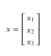
This is a 3D vector along perpendicular axes. This vector would be constructed by travelling x₁, x₂ and x₃ units along their respective axes. This implies that x₁, x₂ and x₃ are scalars.

If you are a victim of how vectors are introduced in Physics ( a la India ), this vector x would be -

Eq.11 : How vector x would be introduced in Physics in the subcontinent

Generalization ramp-up

Say we have a vector y, such that y = f(x), where:

1. x is a vector of size n.
2. y is a vector of m scalar valued functions.

Let’s consider m = n = 3.

Eq.12 : Column vector x, n = 3 (size)

Eq.13 : Column vector y, m = 3 (size)

y is some function of x.

y₁ = f₁(x), which means that y₁ will be some function of x₁, x₂ and x₃.

Let’s define y₁, y₂ and y₃ as follows:

Eq.14 : y₁

Eq.15 : y₂

Eq.16 : y₃

Then the Jacobian of y will be (remember that the Jacobian is simply a stack of the gradients):

Eq.17 : Jacobian of y.

Now, recall that the gradient is simply the matrix of all the partial derivatives:

Eq.18 : Jacobian of y, with the gradients expanded.

We now have a 3 x 3 square Jacobian matrix for this specific case where 𝑥 and 𝑦 both had 3 elements each.

If we consider a more general 𝑦 with m elements:

Eq.19 : A more general Jacobian, where y has a size of m and x has a size of 3.

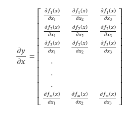
Considering a more general 𝑥. When 𝑥 had 3 dimensions, we had 3 partial derivatives for every scalar function in 𝑦. When 𝑥 has n dimensions, we will have n partial derivatives for every scalar function in 𝑦:

Eq.20 : A more general Jacobian, where y has a size of m and x has a size of n.

The Jacobian is the stack of gradients of a function / vector.
Therefore, we can say that the Jacobian is stack of the all the possible partial derivatives of a vector.
In the above generalized case, the Jacobian is a 𝑚 X 𝑛 matrix.
Each row in the Jacobian is horizontal 𝑛 sized vector.

Jacobian — Analyzing a few cases

For all cases, y = f.

Case 1

Say both f and 𝑥 are scalar. Consider,

Eq.21 : f and x are 1 x 1 scalars.

We know that the Jacobian is the stack of gradients of a vector:

Eq.22 : Generalized Jacobian

But in this case, both f and 𝑥 are scalar, i.e. they are 1x1 matrices. So, the above formula reduces to:

Eq.23 : Jacobian of a scalar with respect to a scalar.

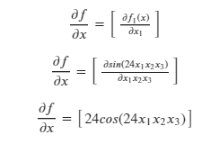
In this case, when f and 𝑥 are both scalar, the Jacobian is also a scalar.

Case 2

Say f is a scalar and 𝑥 is a vector.
x is no longer a 1x1 matrix. Consider:

Eq.24 : f is a 1x1 scalar and x is a 3x1 vector.

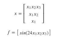
Solving for the Jacobian:

Eq.25 : Jacobian of a scalar with respect to a vector.

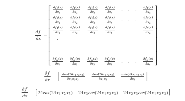
The Jacobian is a matrix in this case, whose dimensions are the transpose of the dimensions of 𝑥.

Case 3

Say 𝑓 is a vector and 𝑥 is a scalar:

Eq.26 : f is a 3x1 vector and x is a 1x1 vector.

Solving for the Jacobian:

Eq.27: Jacobian of a vector with respect to a scalar.

In this case, the Jacobian is a matrix whose dimensions are the same as the dimensions of 𝑓.

Case 4

Say 𝑓 and 𝑥 are both vectors.

Eq.28 : f is a 3x1 vector and x is a 3x1 vector.

Solving for the Jacobian:

Eq.29: Jacobian of a vector with respect to a vector.

In this case the Jacobian is a 𝑚 X 𝑛 matrix where 𝑚 and 𝑛 are dimensions of 𝑓 and 𝑥 respectively.

Summary

To sum up all of the cases mentioned above:

Eq.30 : Variation of Jacobian sizes with input.

That brings us to the end of this post. In the next post in this series, we’ll continue looking at the rest of this paper. Do reach out if you have any comments, questions or suggestions.

Do check out Part 2 of the series.